Analysis of Interferometric Wavefront Data

In this example, we will see how to use prysm to almost entirely supplant the software that comes with a commerical interferometer to analyze the wavefront of an optic. We begin by importing the relevant classes and setting some aesthetics for matplotlib.

from prysm import Interferogram, FringeZernike, sample_files, zernikefit

from matplotlib import pyplot as plt
plt.style.use('bmh')

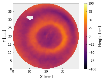
We point prysm to the file, create a new interferogram, mask it to a circular region 100 mm across, subtract piston, tip/tilt and power, and evalute the PV and RMS wavefront error. We also plot the wavefront.

p = sample_files('dat')  # sample Zygo .dat file, will be downloaded on demand and saved locally
i = Interferogram.from_zygo_dat(p)
i.crop().mask('circle', 40).crop()
i.remove_piston_tiptilt_power()
print(i.pv, i.rms)
i.plot2d(clim=100, interpolation='bilinear')  # +/- 100 nm
plt.grid(False)

83.33634959318245 15.245987053549815

The interferogram is cropped twice – once to enclose the valid data, then again to apply a mask centered on that region. For relatively conventional interferometry, you may want to stop here. If you want to use a different unit, that is easy enough,

i.change_z_unit('waves')
1/i.pv, 1/i.rms  # print reciprocal -- "one over xxx waves"

(7.59332515869843, 41.50600402436136)

There is no need to crop again since the outer bound has not changed. Perhaps you wish to evaluated the RMS within the 1 - 10 mm spatial periods,

i.change_z_unit('nm')
i.fill()
i.bandlimited_rms(1,10)

4.440527609280636

This value is derived from the PSD, so you must call fill first. Do not worry about the corners of the array containing data - it will be windowed out. If you do this on a part which has a central obscuration or otherwise departs from being a circle or rectangle, the result will be correct.

If you wish to decompose the wavefront into Zernike polynomials, that is easy enough.

# do this on data which has not been filled to avoid errors introduced by the fill value.
coefficients = zernikefit(i.phase, terms=36, norm=True, map_='Fringe')
fz = FringeZernike(coefficients, dia=i.diameter, z_unit=i.z_unit, norm=True)
print(fz)

rms normalized Fringe Zernike description with:
        -1.195 Z1 - Piston
        -0.543 Z2 - Tilt Y
        -0.944 Z3 - Tilt X
        -3.762 Z4 - Defocus
        -3.688 Z5 - Primary Astigmatism 00°
        -0.662 Z6 - Primary Astigmatism 45°
        -0.615 Z7 - Primary Coma Y
        +4.740 Z8 - Primary Coma X
        -0.539 Z9 - Primary Spherical
        +8.587 Z10 - Primary Trefoil Y
        +3.536 Z11 - Primary Trefoil X
        +5.298 Z12 - Secondary Astigmatism 00°
        +0.587 Z13 - Secondary Astigmatism 45°
        +8.260 Z14 - Secondary Coma Y
        +6.084 Z15 - Secondary Coma X
        +16.659 Z16 - Secondary Spherical
        +4.265 Z17 - Primary Quadrafoil 00°
        +0.526 Z18 - Primary Quadrafoil 45°
        -2.918 Z19 - Secondary Trefoil Y
        -1.598 Z20 - Secondary Trefoil X
        -0.034 Z21 - Tertiary Astigmatism 00°
        -0.398 Z22 - Tertiary Astigmatism 45°
        -4.170 Z23 - Tertiary Coma Y
        -5.492 Z24 - Tertiary Coma X
        -8.338 Z25 - Tertiary Spherical
        +0.593 Z26 - Secondary Pentafoil Y
        -0.264 Z27 - Secondary Pentafoil X
        -0.878 Z28 - Primary Quadrafoil 00°
        -0.171 Z29 - Primary Quadrafoil 45°
        -0.041 Z30 - Tertiary Trefoil Y
        +0.363 Z31 - Tertiary Trefoil X
        -0.437 Z32 - Quaternary Astigmatism 00°
        +0.071 Z33 - Quaternary Astigmatism 45°
        +0.474 Z34 - Quaternary Coma Y
        +0.829 Z35 - Quaternary Coma X
        +1.017 Z36 - Quaternary Spherical
        135.107 PV, 26.483 RMS [nm]

This print might be a bit daunting, one may prefer to see the top few terms by magnitude,

fz.top_n(5)

[(16.659086, 16, 'Secondary Spherical'),
 (8.586951, 10, 'Primary Trefoil Y'),
 (-8.338477, 25, 'Tertiary Spherical'),
 (8.259873, 14, 'Secondary Coma Y'),
 (6.083854, 15, 'Secondary Coma X')]

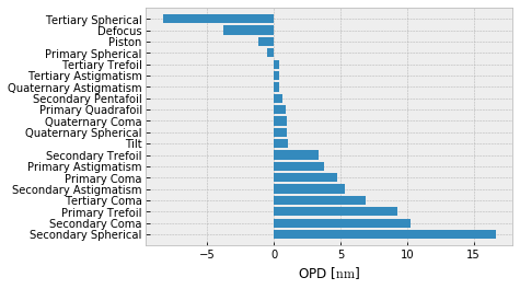
or a barplot of all terms,

fz.barplot_magnitudes(orientation='v', sort=True)

(<Figure size 432x288 with 1 Axes>,
 <matplotlib.axes._subplots.AxesSubplot at 0x7fddac9a86a0>)

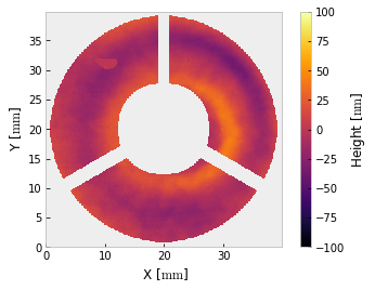
The sample data has a circular clear aperture, but if it had a central obscuration (such as transmitted wavefront data for a telescope) that would be easy to mask too. Here we will build a composite mask for the data as if it were a telescope with an annual aperture disrupted by a spider:

from prysm.geometry import circle, inverted_circle, generate_spider

outer = circle(i.samples_x, radius=1) # radius has units of array semidiameter
inner = inverted_circle(i.samples_x, radius=0.35)

# width has units of arydiam, or pixels if arydiam=None
spider = generate_spider(vanes=3, width=0.5, rotation=90, arydiam=i.diameter, samples=i.samples_x)
mask = outer * inner * spider

i.mask(mask)
i.plot2d(clim=100)  # +/- 100 nm
plt.grid(False)